Important: The GCConnex decommission will not affect GCCollab or GCWiki. Thank you and happy collaborating!
Difference between revisions of "AI-Assisted Quality Control of CTD Data"
| (16 intermediate revisions by the same user not shown) | |||
| Line 1: | Line 1: | ||
| + | ('''Français''': [[Contrôle de la qualité des données CTP assisté par l’IA]]) | ||
As part of the suite of Conductivity, Temperature, Depth (CTD) AI tools being produced by the Office of the Chief Data Steward (OCDS), we are developing a model to assist with identifying and deleting poor-quality scans during the CTD quality control process. Using a combination of a Gaussian Mixture Model (GMM) to cluster CTD scans into groups with similar physical properties and Multi-Layer Perceptrons to classify the scans in each group, we are able to automatically flag the poor-quality scans to be deleted with a high degree of accuracy. Through the deployment of the model as a real-time online endpoint and the support of model communication through a client-side program, we have successfully integrated an experimental model into the client's business process in a field testing environment. The continuation of this line of work will now look to bring the model into a production environment for regular usage in the quality control process. | As part of the suite of Conductivity, Temperature, Depth (CTD) AI tools being produced by the Office of the Chief Data Steward (OCDS), we are developing a model to assist with identifying and deleting poor-quality scans during the CTD quality control process. Using a combination of a Gaussian Mixture Model (GMM) to cluster CTD scans into groups with similar physical properties and Multi-Layer Perceptrons to classify the scans in each group, we are able to automatically flag the poor-quality scans to be deleted with a high degree of accuracy. Through the deployment of the model as a real-time online endpoint and the support of model communication through a client-side program, we have successfully integrated an experimental model into the client's business process in a field testing environment. The continuation of this line of work will now look to bring the model into a production environment for regular usage in the quality control process. | ||
== Use Case Objectives == | == Use Case Objectives == | ||
[[File:Business_process.png|alt=|right|382x382px]] | [[File:Business_process.png|alt=|right|382x382px]] | ||
| − | The quality control process for CTD data is a highly time-intensive task. An oceanographer performs a visual inspection to identify poor-quality scans in each CTD profile using graphical editing software. As the task requires careful inspection and the CTD profiles collected during one year number in the thousands, this work consumes a large amount of time and effort. To ease this burden, we have produced an AI tool that is capable of flagging the poor-quality CTD scans such that these flags can be displayed to the oceanographer within the graphical editing software. This allows for the task to be sped up by providing a quick reference for the areas in the CTD profiles where attention is required. By providing flags for assisted decision-making rather than using the model for fully automated decision-making, we preserve the ability of oceanographer to use their domain expertise to make the best possible decisions. As the model becomes more mature and its performance improves, we may explore options to increase the degree of automation. | + | The quality control process for CTD data is a highly time-intensive task. An oceanographer performs a visual inspection to identify poor-quality scans in each CTD profile using graphical editing software. As the task requires careful inspection of the data and the CTD profiles collected during one year number in the thousands, this work consumes a large amount of time and effort. To ease this burden, we have produced an AI tool that is capable of flagging the poor-quality CTD scans such that these flags can be displayed to the oceanographer within the graphical editing software. This allows for the task to be sped up by providing a quick reference for the areas in the CTD profiles where attention is required. By providing flags for assisted decision-making rather than using the model for fully automated decision-making, we preserve the ability of oceanographer to use their domain expertise to make the best possible decisions. As the model becomes more mature and its performance improves, we may explore options to increase the degree of automation. |
* '''Machine Learning Task''': Flag in advance the scans to be deleted during CTD quality control | * '''Machine Learning Task''': Flag in advance the scans to be deleted during CTD quality control | ||
| − | * '''Business Value''': Flagged scans allow the | + | * '''Business Value''': Flagged scans allow the oceanographer to quickly focus attention on crucial areas, reducing the time and effort required to delete scans |
* '''Measures of Success''': | * '''Measures of Success''': | ||
** Accuracy of model predictions | ** Accuracy of model predictions | ||
| Line 25: | Line 26: | ||
The data partitioning step is used to break the CTD scans up into groups that have similar physical properties to each other. Since the CTD profiles are collected across a vast geographical area (the North-East Pacific), a large span of depths (0 to 4300 meters below surface) and across all seasons, these spatio-temporal variations lead to a highly varied distribution of physical properties in the CTD scans. This degree of variation is difficult for a single MLP to cope with and learn how to distinguish between good or poor-quality scans in all observed conditions. Performance can be greatly improved by first partitioning the scans and then training a separate MLP for each partition. We achieve this using a GMM trained on the primary physical properties of the scans, namely the temperature, conductivity and salinity values. | The data partitioning step is used to break the CTD scans up into groups that have similar physical properties to each other. Since the CTD profiles are collected across a vast geographical area (the North-East Pacific), a large span of depths (0 to 4300 meters below surface) and across all seasons, these spatio-temporal variations lead to a highly varied distribution of physical properties in the CTD scans. This degree of variation is difficult for a single MLP to cope with and learn how to distinguish between good or poor-quality scans in all observed conditions. Performance can be greatly improved by first partitioning the scans and then training a separate MLP for each partition. We achieve this using a GMM trained on the primary physical properties of the scans, namely the temperature, conductivity and salinity values. | ||
| − | Finally, data classification is achieved using | + | Finally, data classification is achieved using one MLP per cluster of CTD scans. The MLP is trained for binary classification to flag CTD scans as poor-quality (to be deleted) or good quality (to be preserved). The ground truth used to produce the training data is derived from historical instances of quality control, using the decisions made by oceanographers in the past regarding which scans should be deleted. The deleted scans are far fewer than the preserved scans, making the training data highly imbalanced. This is often problematic in a machine learning setting as it causes the model to learn in a fashion biased towards the majority class. To address this, we apply oversampling to randomly duplicate deleted scans in the training data in order to balance their numbers with the preserved scans. |
[[File:Ml_pipeline.png|alt=|center|992x992px]] | [[File:Ml_pipeline.png|alt=|center|992x992px]] | ||
| − | |||
| − | |||
| − | |||
| − | |||
| − | |||
==Experimental Model Performance== | ==Experimental Model Performance== | ||
[[File:Performance.png|alt=|right|477x477px]] | [[File:Performance.png|alt=|right|477x477px]] | ||
| Line 42: | Line 38: | ||
It is also important to note that the quality of the model flags is impacted by the depth of the scans being processed. The shallowest depths are the most difficult to handle as the greatest variations in the physical properties of the water occur near the surface. A breakdown of model performance by depth ranges can be seen in the figure on the right. The first 50 meters are quite challenging, resulting in a model accuracy of roughly 88.7%. While the scans beneath 500 meters are more regular, resulting in a model accuracy of roughly 94.1%. | It is also important to note that the quality of the model flags is impacted by the depth of the scans being processed. The shallowest depths are the most difficult to handle as the greatest variations in the physical properties of the water occur near the surface. A breakdown of model performance by depth ranges can be seen in the figure on the right. The first 50 meters are quite challenging, resulting in a model accuracy of roughly 88.7%. While the scans beneath 500 meters are more regular, resulting in a model accuracy of roughly 94.1%. | ||
| − | + | Perfect model accuracy will never be obtainable as there is uncertainty in the decision-making even for oceanographers. There are many complex factors at play influencing the data that is ultimately recorded such as choppy water causing the scanning equipment to descend irregularly, winds and strong weather conditions causing mixing of waters near the surface, and currents causing mixing of waters under the surface. As the distinction between proper and corrupted scan data can be very difficult to identify under these conditions, the human decision-making process is not guaranteed to be perfect. This in fact highlights a potential area where the development of more mature AI models that can exploit additional information on these factors may have the potential to lead to automated approaches that could eventually augment the human decisions to a higher overall quality. | |
| − | |||
| + | |||
| Line 51: | Line 47: | ||
==Model Deployment and Integration== | ==Model Deployment and Integration== | ||
To get practical value out of the AI model, it must be integrated into the client's business process in an easy-to-use manner. We have taken the approach of making the model available via a real-time online endpoint deployed on a cloud analytics platform. The client then uses the model through communication with the endpoint managed by a client-side program which runs on the user's machine. | To get practical value out of the AI model, it must be integrated into the client's business process in an easy-to-use manner. We have taken the approach of making the model available via a real-time online endpoint deployed on a cloud analytics platform. The client then uses the model through communication with the endpoint managed by a client-side program which runs on the user's machine. | ||
| − | |||
| − | + | For the field test setting, we have used Azure Databricks as the cloud analytics platform through which the model is deployed. A real-time online endpoint is used to make the model available via an Application Programming Interface (API). This means that authenticated users can access the model from any machine that is connected to the internet. We have produced a light-weight client-side program that runs on the user's machine to manage communication with the model. This program provides a simple graphical interface used to select the CTD files to send to the model for processing. The program then receives a response with the flags generated by the model and saves new files containing the results. These files can be loaded directly into the graphical editor used during the standard CTD quality control process. This provides the user with a simple method to use the model with minimal overhead and integrates the model results directly into the existing quality control software. | |
| − | [[File:Model_communications.png|alt=|center]] | + | The user can optionally send the CTD files back to the model endpoint after the quality control process has been finished. This allows for the scan deletion decisions made by the user to be compared against the model's predicted flags in order to assess the performance of the model. The results are then analyzed to provide a breakdown of the model performance across various metrics which are presented visually in a Power BI report.[[File:Model_communications.png|alt=|center]] |
| Line 62: | Line 57: | ||
==Next Steps == | ==Next Steps == | ||
| + | Having gone through the proof-of-concept and field test stages, the model has demonstrated positive results that can lead to business value by speeding up the CTD quality control process. We are now in a position to begin preparations to bring the model into a production environment. Refinements to the model deployment, integration architecture and backing code will be implemented to ensure that the model functionality can be supplied to the client in the form of a robust tool. Monitoring must also be implemented to ensure that the model continues to deliver reliable performance over time. If model drift is detected during monitoring, this must trigger corrective action to retrain the model. Finally, an in-depth model reporting dashboard will be designed to provide detailed information on model performance, enabling the user to better understand the tool they are working with. | ||
Latest revision as of 16:59, 10 January 2023
(Français: Contrôle de la qualité des données CTP assisté par l’IA)
As part of the suite of Conductivity, Temperature, Depth (CTD) AI tools being produced by the Office of the Chief Data Steward (OCDS), we are developing a model to assist with identifying and deleting poor-quality scans during the CTD quality control process. Using a combination of a Gaussian Mixture Model (GMM) to cluster CTD scans into groups with similar physical properties and Multi-Layer Perceptrons to classify the scans in each group, we are able to automatically flag the poor-quality scans to be deleted with a high degree of accuracy. Through the deployment of the model as a real-time online endpoint and the support of model communication through a client-side program, we have successfully integrated an experimental model into the client's business process in a field testing environment. The continuation of this line of work will now look to bring the model into a production environment for regular usage in the quality control process.
Use Case Objectives
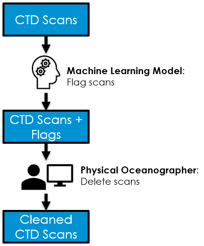
The quality control process for CTD data is a highly time-intensive task. An oceanographer performs a visual inspection to identify poor-quality scans in each CTD profile using graphical editing software. As the task requires careful inspection of the data and the CTD profiles collected during one year number in the thousands, this work consumes a large amount of time and effort. To ease this burden, we have produced an AI tool that is capable of flagging the poor-quality CTD scans such that these flags can be displayed to the oceanographer within the graphical editing software. This allows for the task to be sped up by providing a quick reference for the areas in the CTD profiles where attention is required. By providing flags for assisted decision-making rather than using the model for fully automated decision-making, we preserve the ability of oceanographer to use their domain expertise to make the best possible decisions. As the model becomes more mature and its performance improves, we may explore options to increase the degree of automation.
- Machine Learning Task: Flag in advance the scans to be deleted during CTD quality control
- Business Value: Flagged scans allow the oceanographer to quickly focus attention on crucial areas, reducing the time and effort required to delete scans
- Measures of Success:
- Accuracy of model predictions
- Client feedback on quality control speed-ups
- Aspirational Goals:
- Mitigation of uncertainty in human decisions
- Semi or full automation of scan deletions
Machine Learning Pipeline
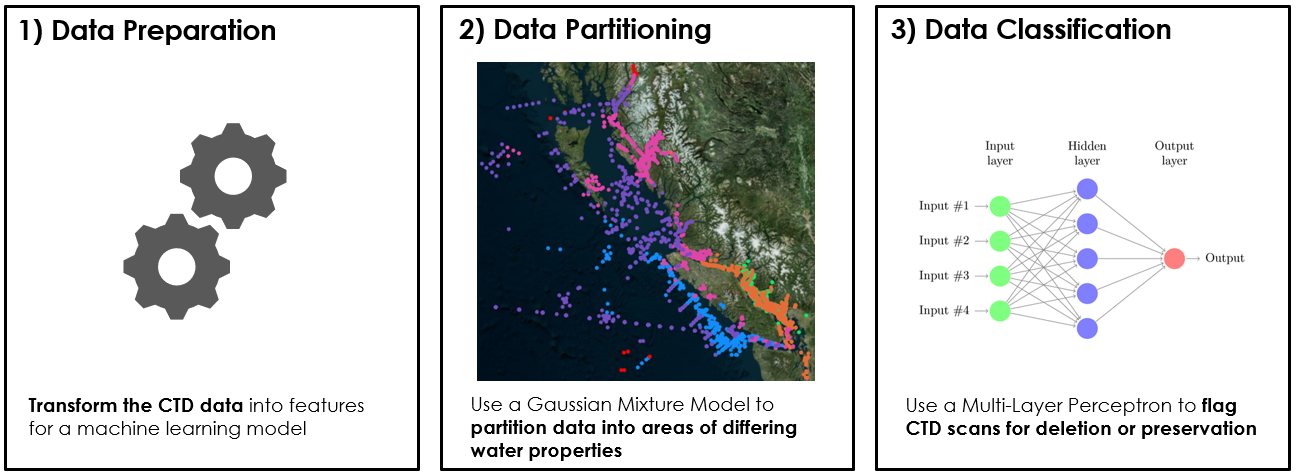
The machine learning pipeline consists of three main steps: data preparation, data partitioning via a Gaussian Mixture Model (GMM) and data classification via a Multi-Layer Perceptron (MLP).
The data preparation covers the standard machine learning tasks of data cleaning, feature engineering and scaling. The feature engineering is used to draw out the most relevant information from the data for later use in the classification task. The MLP classifies each CTD scan independently based on its features. However, the local neighborhood around each scan often contains valuable information about the changes of feature values across the depth-wise dimension of the CTD profile and the rate at which these values are changing. Sudden rapid changes in values can be strong indicators of factors corrupting the data recorded in the CTD scans. We therefore place windows of various sizes around each CTD scan and calculate statistics over the scan values within the window to augment each CTD scan with information about different sized local neighborhoods. Our experimental evaluations have shown these additional features to have a positive impact on the performance of the model.
The data partitioning step is used to break the CTD scans up into groups that have similar physical properties to each other. Since the CTD profiles are collected across a vast geographical area (the North-East Pacific), a large span of depths (0 to 4300 meters below surface) and across all seasons, these spatio-temporal variations lead to a highly varied distribution of physical properties in the CTD scans. This degree of variation is difficult for a single MLP to cope with and learn how to distinguish between good or poor-quality scans in all observed conditions. Performance can be greatly improved by first partitioning the scans and then training a separate MLP for each partition. We achieve this using a GMM trained on the primary physical properties of the scans, namely the temperature, conductivity and salinity values.
Finally, data classification is achieved using one MLP per cluster of CTD scans. The MLP is trained for binary classification to flag CTD scans as poor-quality (to be deleted) or good quality (to be preserved). The ground truth used to produce the training data is derived from historical instances of quality control, using the decisions made by oceanographers in the past regarding which scans should be deleted. The deleted scans are far fewer than the preserved scans, making the training data highly imbalanced. This is often problematic in a machine learning setting as it causes the model to learn in a fashion biased towards the majority class. To address this, we apply oversampling to randomly duplicate deleted scans in the training data in order to balance their numbers with the preserved scans.
Experimental Model Performance
In order to validate the performance of the model, we have performed experimentation using historical CTD data covering the years 2013-2021. We use a 5-fold cross-validation methodology to ensure robustness in the measured results.
It is important that the model is able to effectively classify both the scans to be deleted as well as the scans to be preserved, or in the context of machine learning, the positive and negative samples. While the performance for classification of positive and negative samples can be measured separately, we have configured the model to balance performance across these two goals. Therefore, we report only the overall accuracy of the model here for simplicity. The global accuracy achieved by the model is roughly 92.6% measured against the historical decisions made by oceanographers. This demonstrates that the model has learned to effectively observe the patterns indicative of poor-quality scans and replicate the decision-making used by oceanographers with a high degree of accuracy.
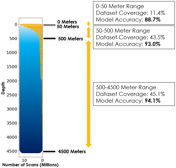
It is also important to note that the quality of the model flags is impacted by the depth of the scans being processed. The shallowest depths are the most difficult to handle as the greatest variations in the physical properties of the water occur near the surface. A breakdown of model performance by depth ranges can be seen in the figure on the right. The first 50 meters are quite challenging, resulting in a model accuracy of roughly 88.7%. While the scans beneath 500 meters are more regular, resulting in a model accuracy of roughly 94.1%.
Perfect model accuracy will never be obtainable as there is uncertainty in the decision-making even for oceanographers. There are many complex factors at play influencing the data that is ultimately recorded such as choppy water causing the scanning equipment to descend irregularly, winds and strong weather conditions causing mixing of waters near the surface, and currents causing mixing of waters under the surface. As the distinction between proper and corrupted scan data can be very difficult to identify under these conditions, the human decision-making process is not guaranteed to be perfect. This in fact highlights a potential area where the development of more mature AI models that can exploit additional information on these factors may have the potential to lead to automated approaches that could eventually augment the human decisions to a higher overall quality.
Model Deployment and Integration
To get practical value out of the AI model, it must be integrated into the client's business process in an easy-to-use manner. We have taken the approach of making the model available via a real-time online endpoint deployed on a cloud analytics platform. The client then uses the model through communication with the endpoint managed by a client-side program which runs on the user's machine.
For the field test setting, we have used Azure Databricks as the cloud analytics platform through which the model is deployed. A real-time online endpoint is used to make the model available via an Application Programming Interface (API). This means that authenticated users can access the model from any machine that is connected to the internet. We have produced a light-weight client-side program that runs on the user's machine to manage communication with the model. This program provides a simple graphical interface used to select the CTD files to send to the model for processing. The program then receives a response with the flags generated by the model and saves new files containing the results. These files can be loaded directly into the graphical editor used during the standard CTD quality control process. This provides the user with a simple method to use the model with minimal overhead and integrates the model results directly into the existing quality control software.
The user can optionally send the CTD files back to the model endpoint after the quality control process has been finished. This allows for the scan deletion decisions made by the user to be compared against the model's predicted flags in order to assess the performance of the model. The results are then analyzed to provide a breakdown of the model performance across various metrics which are presented visually in a Power BI report.
Next Steps
Having gone through the proof-of-concept and field test stages, the model has demonstrated positive results that can lead to business value by speeding up the CTD quality control process. We are now in a position to begin preparations to bring the model into a production environment. Refinements to the model deployment, integration architecture and backing code will be implemented to ensure that the model functionality can be supplied to the client in the form of a robust tool. Monitoring must also be implemented to ensure that the model continues to deliver reliable performance over time. If model drift is detected during monitoring, this must trigger corrective action to retrain the model. Finally, an in-depth model reporting dashboard will be designed to provide detailed information on model performance, enabling the user to better understand the tool they are working with.


